Create a phase curve#
squishyplanet can also model phase curves of triaxial planets, however, here it uses a numerical 2D Monte Carlo approach instead of the faster/more accurate 1D integrals it solves with quadrature methods when computing the planet’s transit lightcurve. This is both slow and memory intensive but does in theory provide for some flexibility to choose interesting reflection/emission laws. Pre-version 1.0, squishyplanet only supports uniform albedo Lambertian scattering for reflections and a
single hotspot modeled by a von Mises-Fisher distribution for thermal emission, though hopefully more options will be added in the future. Fingers crossed that eventually we’ll abandon this approach altogether and implement a spherical harmonic expansion of the emission and reflection maps, which we then can integrate again with 1D methods à la starry.
squishyplanet handles secondary eclipses by masking each sample of the surface according to whether it’s behind the star or not. Consquently, these should be about as accurate as the rest of the phase curve.
Finally, squishyplanet can include two effects on the phase curve sourced from the star, not the planet: ellipsoidal variations and stellar doppler beaming. However, it does so using simple models that do not attempt to capture the full, complicated physical picture of the moving, gravity-darkened star. Instead, they are modeled as sinusoids with periods of twice and equal to the orbital period, respectively. These are scaled by a user-provided amplitude (or fitted) amplitude: these
amplitudes are related to other parameters in the model (e.g. Wong et al. 2020), but it’s up to the user to include those relationships in a prior if they wish.
[1]:
import jax

jax.config.update("jax_enable_x64", True)
import jax.numpy as jnp
import matplotlib.pyplot as plt
import numpy as np
import astropy.units as u
import astropy.constants as const

from squishyplanet import OblateSystem
Reflections#
First we’ll demonstrate how you can use squishyplanet to model the contributions of reflected light to a phase curve. We first have to set compute_reflected_phase_curve to True, then set a value for albedo. Again, squishyplanet will assume the planet is a Lambertian reflector with a uniform albedo across its surface. It will correctly handle the non-spherical geometry of the planet, however.
[2]:
state = {
    "t_peri": -0.25,
    "times": jnp.linspace(-0.6, 0.6, 500),
    "a": 5.0,
    "period": 1.0,
    "r": 0.1,
    "i": jnp.pi / 2,
    "ld_u_coeffs": jnp.array([0.4, 0.26]),
    "tidally_locked": False,
    "compute_reflected_phase_curve": True,
    "albedo": 0.2,
}
planet = OblateSystem(**state)

fig, ax = plt.subplots()
ax.plot(planet.state["times"], planet.lightcurve())
w = 3e-4
ax.set(ylim=[1 - 3e-4, 1 + 1e-4], xlabel="Time", ylabel="Flux");
At each timestep in this curve, we perform a Monte Carlo estimate to measure the amount of reflected light. To estimate the noise/bias introduced this procedure, we can create an identical system with a different random seed and compare the two estimates:
[3]:
state = {
    "t_peri": -0.25,
    "times": jnp.linspace(-0.6, 0.6, 500),
    "a": 5.0,
    "period": 1.0,
    "r": 0.1,
    "i": jnp.pi / 2,
    "ld_u_coeffs": jnp.array([0.4, 0.26]),
    "tidally_locked": False,
    "compute_reflected_phase_curve": True,
    "albedo": 0.2,
    "random_seed": 0,
}
planet1 = OblateSystem(**state)

state["random_seed"] = 1
planet2 = OblateSystem(**state)

diff = planet1.lightcurve() - planet2.lightcurve()

fig, ax = plt.subplots()
ax.plot(planet1.state["times"], diff * 1e6)
ax.set(xlabel="Time", ylabel="Flux difference [ppm]");
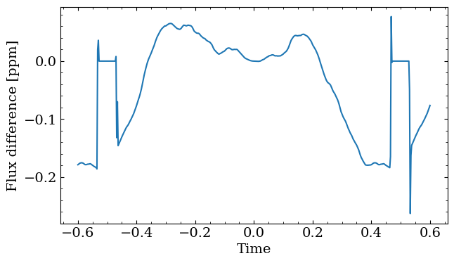
In this example, it looks like the noise is acceptable/sub-ppm when using the default settings, which use 50,000 samples per timestep. We can achieve ppm-level differences with comparatively small number of samples since we use the Monte Carlo integration to calculate the fraction of reflected light, not the absolute amount. The results of our estimate are scaled by the projected size of the planet and the distance to the star, so even ~ppt level accuracy in the Monte Carlo estimate will result in ppm-level accuracy in the phase curve.
We can compare our reflect curves of spherical planets with starry’s estimate of the same system. Since as of writing starry is difficult to install due to some dependency conflicts, we pre-generated this curve using starry v1.2.0:
[4]:
# import astropy.units as u
# import astropy.constants as const
# import numpy as np
# import matplotlib.pyplot as plt
# import starry
# starry.config.lazy = False
# starry.config.quiet = True
# star_mass = ((5.0*u.R_sun)**3 / (1.0*u.day)**2 / (const.G) * (4*np.pi**2)).to(u.M_sun).value
# starry.config.lazy = False
# starry.config.quiet = True
# sun = starry.Primary(starry.Map(), r=1, length_unit=u.Rsun, m=star_mass, m_unit=u.Msun)
# map = starry.Map(reflected=True)
# planet = starry.Secondary(map, a=5.0, m=0.0, inc=90, r=0.1, length_unit=u.Rsun)
# planet.map.amp = 0.2
# sys = starry.System(sun, planet)
# np.save("starry_reflected_curve.npy", sys.flux(t))

starry_flux = np.load("starry_reflected_curve.npy")


state = {
    "t_peri": -0.25,
    "times": jnp.linspace(-0.6, 0.6, 500),
    "a": 5.0,
    "period": 1.0,
    "r": 0.1,
    "i": jnp.pi / 2,
    "ld_u_coeffs": jnp.array([0.0, 0.0]),
    "tidally_locked": False,
    "compute_reflected_phase_curve": True,
    "albedo": 0.2,
}
planet = OblateSystem(**state)
lc = planet.lightcurve()

fig, axs = plt.subplots(nrows=2, figsize=(8, 10), sharex=True)
axs[0].plot(planet.state["times"], lc, label="squishyplanet")
axs[0].plot(planet.state["times"], starry_flux, ls="--", label="starry")
w = 3e-4
axs[0].set(ylim=[1 - 3e-4, 1 + 1e-4], xlabel="Time", ylabel="Flux")
axs[0].legend()

axs[1].plot(planet.state["times"], 1e6 * (lc - starry_flux))
axs[1].set(xlabel="Time", ylabel="Flux difference [ppm]")

fig.subplots_adjust(hspace=0);
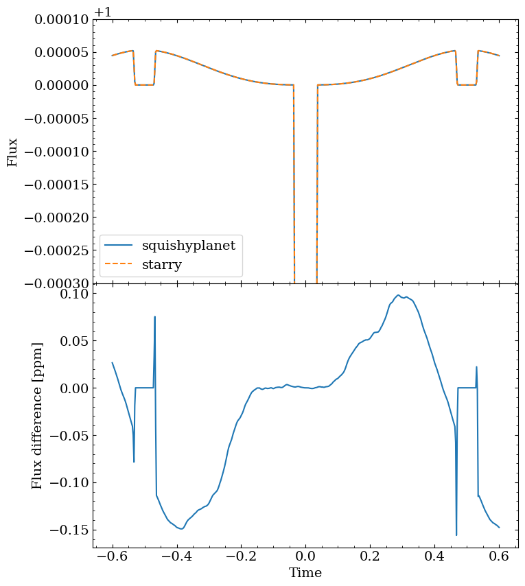
Again, the differences are sub-ppm.
Emission only#
Adding emission to the phase curve looks very similar to adding reflection. For now, squishyplanet only allows for thermal maps with a single hotspot that are modeled with a von Mises-Fisher distribution. To mimic an isothermal planet, we can set the hotspot_concentration to a very low value.
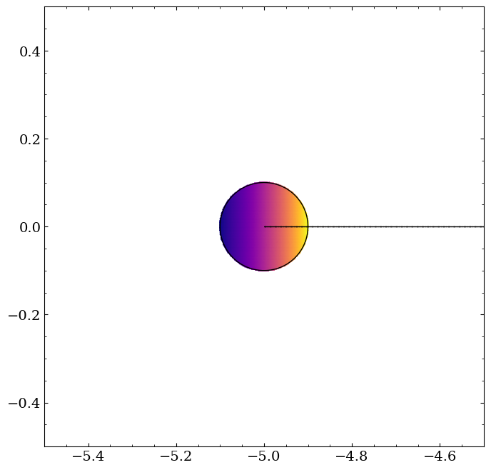
Here we have to set compute_emission_phase_curve to True, then set a values for hotspot_latitude, hotspot_longitude, and hotspot_concentration. The concentration is the kappa parameter of the von Mises-Fisher distribution. We can use the .illustrate method to visualize the hotspot on the planet’s surface:
[5]:
state = {
    "t_peri": -0.25,
    "times": jnp.linspace(-0.6, 0.6, 500),
    "a": 5.0,
    "period": 1.0,
    "r": 0.1,
    "i": jnp.pi / 2,
    "ld_u_coeffs": jnp.array([0.4, 0.26]),
    "tidally_locked": True,
    "compute_emitted_phase_curve": True,
    "hotspot_longitude": 0.0,
    "hotspot_latitude": -jnp.pi/2,
    "hotspot_concentration": 0.5,
    "emitted_scale" : 1e-4,
}
planet = OblateSystem(**state)

planet.illustrate(emitted=True, window_size=1, star_fill=False, true_anomalies=0.0)
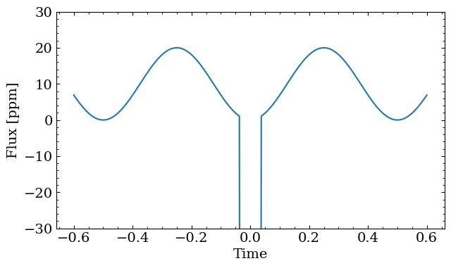
[6]:
lc = planet.lightcurve()
fig, ax = plt.subplots()
ax.plot(planet.state["times"], (lc-1)*1e6)
w = 300
ax.set(xlabel="Time", ylabel="Flux [ppm]", ylim=[-w, w]);
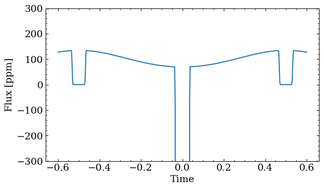
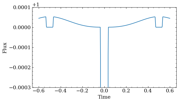
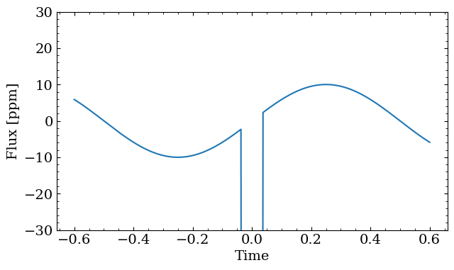
We can also look at the impact of shifting the hotspot longitude away from the sub-stellar point:
[7]:
sub_solar = planet.lightcurve()
shifted = planet.lightcurve({"hotspot_longitude": 20*jnp.pi/180})

fig, axs = plt.subplots(nrows=2, figsize=(8, 10), sharex=True)
axs[0].plot(planet.state["times"], (sub_solar-1)*1e6, label="sub-solar hotspot")
axs[0].plot(planet.state["times"], (shifted-1)*1e6, ls="--", label="shifted hotspot")
axs[0].set(ylim=[-300, 300], xlabel="Time", ylabel="Flux")

axs[1].plot(planet.state["times"], 1e6 * (sub_solar - shifted))
axs[1].set(xlabel="Time", ylabel="Flux difference [ppm]")

fig.subplots_adjust(hspace=0);
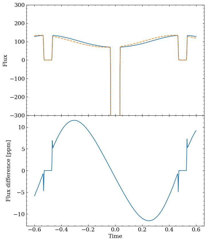
The result is a sinusoidal difference between the two curves, plus some differences during ingress/egress of secondary eclipse. The curves agree nearly perfectly when the planet is fully blocked by the star, as expected, but still differ during primary transit. That’s because their flux-blocking areas are identical, but their night-side emission is different.
Stellar effects#
squishyplanet can also include two types of deviations to a standard phase curve caused by the star, not by the planet. Each of these calculations assume the planet is on a circular orbit. The first of these are “ellipsoidal variations”, or variations you get from the planet’s gravitational influence. This produces a sinusoidal variation with a period of half the orbital period: the hemispheres directly facing and directly opposite the planet are darker compared to the bits that are 90
degrees away from the sub-planet point in longitude:
[8]:
state = {
    "t_peri": -0.25,
    "times": jnp.linspace(-0.6, 0.6, 500),
    "a": 5.0,
    "period": 1.0,
    "r": 0.1,
    "i": jnp.pi / 2,
    "ld_u_coeffs": jnp.array([0.4, 0.26]),
    "tidally_locked": True,
    "compute_stellar_ellipsoidal_variations": True,
    "stellar_ellipsoidal_alpha":1e-5,
}
planet = OblateSystem(**state)

lc = planet.lightcurve()
fig, ax = plt.subplots()
ax.plot(planet.state["times"], (lc-1)*1e6)
w = 30
ax.set(xlabel="Time", ylabel="Flux [ppm]", ylim=[-w, w]);
Note we don’t see a secondary eclipse here since we’ve left compute_emitted_phase_curve and compute_reflected_phase_curve as False.
The second effect is the “beaming” effect, which is a relativistic effect that causes the star to appear brighter when it’s moving towards us and dimmer when it’s moving away. This effect is also sinusoidal, but with a period equal to the orbital period:
[9]:
state = {
    "t_peri": -0.25,
    "times": jnp.linspace(-0.6, 0.6, 500),
    "a": 5.0,
    "period": 1.0,
    "r": 0.1,
    "i": jnp.pi / 2,
    "ld_u_coeffs": jnp.array([0.4, 0.26]),
    "tidally_locked": True,
    "compute_stellar_doppler_variations": True,
    "stellar_doppler_alpha":1e-5,
}
planet = OblateSystem(**state)

lc = planet.lightcurve()
fig, ax = plt.subplots()
ax.plot(planet.state["times"], (lc-1)*1e6)
w = 30
ax.set(xlabel="Time", ylabel="Flux [ppm]", ylim=[-w, w]);
Here the star is dimmer as it moves away, then brighter as it moves towards, the observer. Note that squishyplanet follows the typical transiting planet convention and sets \(\Omega=\pi\) by default, so that a planet on a circular orbit transits at \(f=\pi/2\) as it moves from left to right across the sky plane.
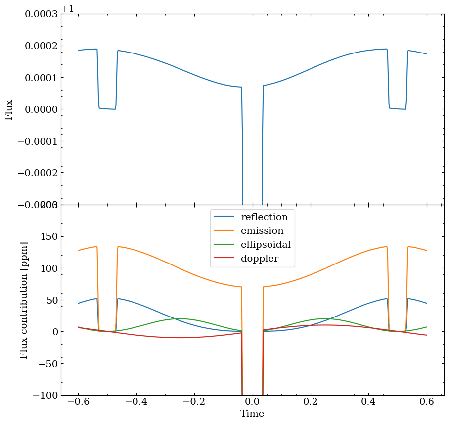
All combined#
[10]:
state = {
    "t_peri": -0.25,
    "times": jnp.linspace(-0.6, 0.6, 500),
    "a": 5.0,
    "period": 1.0,
    "r": 0.1,
    "i": jnp.pi / 2,
    "ld_u_coeffs": jnp.array([0.4, 0.26]),
    "tidally_locked": True,
    "compute_reflected_phase_curve": True,
    "compute_emitted_phase_curve": True,
    "compute_stellar_ellipsoidal_variations": True,
    "compute_stellar_doppler_variations": True,
    "albedo": 0.2,
    "hotspot_longitude": 0.0,
    "hotspot_latitude": -jnp.pi/2,
    "hotspot_concentration": 0.5,
    "emitted_scale" : 1e-4,
    "stellar_ellipsoidal_alpha":1e-5,
    "stellar_doppler_alpha":1e-5,
    "random_seed": 0,
}

planet = OblateSystem(**state)
lc = planet.lightcurve()

fig, axs = plt.subplots(nrows=2, figsize=(10, 10), sharex=True)
axs[0].plot(planet.state["times"], lc)
w = 3e-4
axs[0].set(ylim=[1 - w, 1 + w], ylabel="Flux")


zeroed_out = {
    "albedo": 0.0,
    "emitted_scale": 0.0,
    "stellar_ellipsoidal_alpha": 0.0,
    "stellar_doppler_alpha": 0.0,
}
reflection_only = zeroed_out.copy()
reflection_only["albedo"] = 0.2
axs[1].plot(planet.state["times"], (planet.lightcurve(reflection_only)-1)*1e6, label="reflection")

emission_only = zeroed_out.copy()
emission_only["emitted_scale"] = 1e-4
axs[1].plot(planet.state["times"], (planet.lightcurve(emission_only)-1)*1e6, label="emission")

ellipsoidal_only = zeroed_out.copy()
ellipsoidal_only["stellar_ellipsoidal_alpha"] = 1e-5
axs[1].plot(planet.state["times"], (planet.lightcurve(ellipsoidal_only)-1)*1e6, label="ellipsoidal")

doppler_only = zeroed_out.copy()
doppler_only["stellar_doppler_alpha"] = 1e-5
axs[1].plot(planet.state["times"], (planet.lightcurve(doppler_only)-1)*1e6, label="doppler")

axs[1].legend()
axs[1].set(xlabel="Time", ylabel="Flux contribution [ppm]", ylim=[-100, 200])

fig.subplots_adjust(hspace=0);