Transits of ringed planets

squishyplanet can model transits of planets that host an opaque ring via the RingedSystem class. The ring is assumed to be:

• perfectly flat and infinitely thin,

• perfectly circular and concentric with the planet,

• perfectly opaque,

• bounded by an inner radius ring_inner_r and an outer radius ring_outer_r, both in units of the stellar radius. The inner radius must be larger than the planet’s equatorial radius r.

By default the ring lies in the planet’s equatorial plane: its 3D orientation follows the planet’s obliq and prec angles, including the time-varying orientation of a tidally locked planet (though we likely wouldn’t expect such a configuration). You can decouple the ring from the planet by passing ring_obliq and ring_prec explicitly.

The flux blocked by the combined planet + ring silhouette is computed with the same Green’s theorem boundary integrals used for the planet alone, so it inherits support for arbitrary-order polynomial limb darkening laws and is exact up to quadrature/root-finding precision. That includes the awkward configurations where the planet’s disk overlaps the projected ring edges, or where a nearly edge-on ring crosses the stellar limb four times: no small-planet or non-overlapping approximations are involved. See the changelog and the engine.ringed_transit module documentation for details on the algorithm.

import jax

jax.config.update("jax_enable_x64", True)
import jax.numpy as jnp
import matplotlib.pyplot as plt

from squishyplanet import OblateSystem, RingedSystem

Creating a RingedSystem

RingedSystem is a subclass of OblateSystem and accepts all of the same arguments (see the Quickstart), plus the four ring parameters. Let’s set up a Saturn-like planet on a circular orbit. Note that with t_peri = -period / 4, a circular orbit with the default omega and Omega reaches mid-transit at \(t=0\).

One thing to point out: the planet below is a sphere, so its own obliq and prec don’t affect its outline at all. But since we don’t pass ring_obliq or ring_prec, the ring lies in the equatorial plane those angles define, and they shape the transit through the ring alone.

state = {
    "times": jnp.linspace(-0.75, 0.75, 500),  # days
    "t_peri": -2.5,
    "period": 10.0,
    "a": 5.0,
    "i": jnp.pi / 2 - 0.01,
    "r": 0.1,
    "obliq": 0.4,
    "prec": jnp.pi / 2,
    "tidally_locked": False,
    "ld_u_coeffs": jnp.array([0.3, 0.1]),
}

ringed = RingedSystem(ring_inner_r=0.15, ring_outer_r=0.3, **state)
planet_only = OblateSystem(**state)

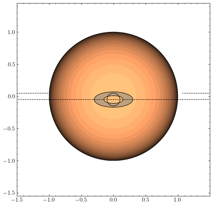
RingedSystem.illustrate works just like OblateSystem.illustrate, but overlays the projected outlines of both ring edges and (optionally, controlled by ring_fill) fills the annulus between them. One caveat noted in its docstring: the layering is cosmetic, so the filled annulus is drawn on top of the planet even though half of the physical ring passes behind it.

ringed.illustrate(times=jnp.array([0.0]), window_size=3.0)

The lightcurve

Generating a lightcurve is identical to the OblateSystem case:

lc_ringed = ringed.lightcurve()
lc_planet = planet_only.lightcurve()

fig, ax = plt.subplots(figsize=(8, 4))
ax.plot(state["times"], lc_planet, label="planet only")
ax.plot(state["times"], lc_ringed, label="planet + ring")
ax.set(xlabel="Time [days]", ylabel="Relative flux")
ax.legend();

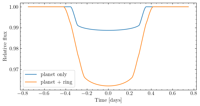
The ring both deepens the transit (it blocks extra area) and lengthens it (the outer ring edge reaches the stellar limb well before the planet does), and it reshapes ingress/egress: the initial shallow slopes are the annulus sliding onto the star, followed by the steeper drop of the planet itself.

Changing the ring’s orientation

To orient the ring independently of the planet, pass both ring_obliq and ring_prec (defined identically to the planet’s obliq and prec; see the geometry visualizations). The projected annulus depends on how the ring plane is tilted relative to the line of sight, and some care is needed: for example, for an exactly edge-on orbit (\(i = \pi/2\)), a ring with ring_prec = 0 presents itself perfectly edge-on for any value of ring_obliq and blocks no light at all.

Like every other model parameter, the ring parameters can be updated at call time by passing a dictionary to lightcurve – this is the same mechanism you would use when fitting data. Here is a family of models where only the ring’s obliquity changes:

decoupled = RingedSystem(
    ring_inner_r=0.15,
    ring_outer_r=0.3,
    ring_obliq=0.2,
    ring_prec=jnp.pi / 2,
    **state,
)

fig, ax = plt.subplots(figsize=(8, 4))
for ring_obliq in [0.05, 0.3, 0.7, jnp.pi / 2]:
    lc = decoupled.lightcurve({"ring_obliq": jnp.array([ring_obliq])})
    ax.plot(state["times"], lc, label=f"ring_obliq = {ring_obliq:.2f}")
ax.set(xlabel="Time [days]", ylabel="Relative flux")
ax.legend();

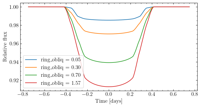
We can also visualize these 4 geometries by creating a new RingedSystem for each one and calling illustrate. Note that we don’t need to create new objects to generate lightcurves, but we do just for illustrations since it relies on some internal state created at object initialization.

for ring_obliq in [0.05, 0.3, 0.7, jnp.pi / 2]:
    s = state.copy()
    s["obliq"] = ring_obliq
    ringed = RingedSystem(ring_inner_r=0.15, ring_outer_r=0.3, **s)
    ringed.illustrate(window_size=3.0)

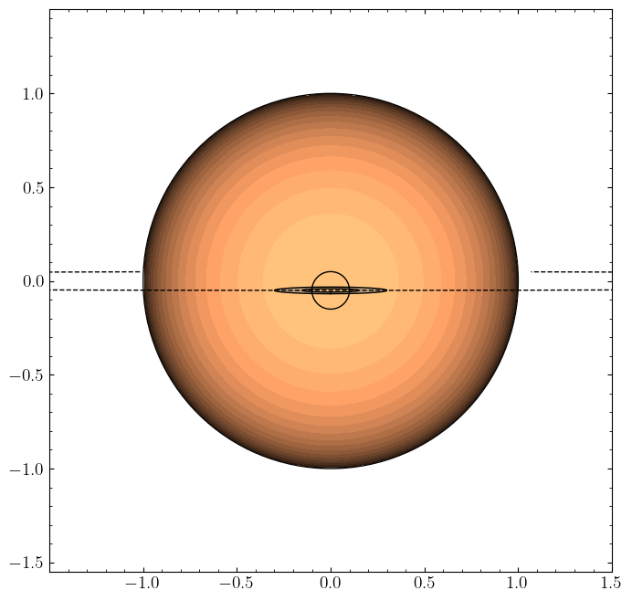
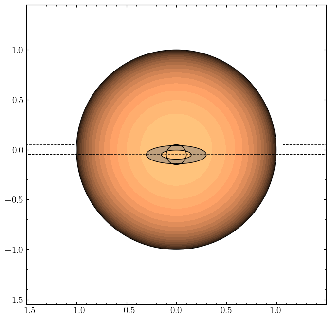
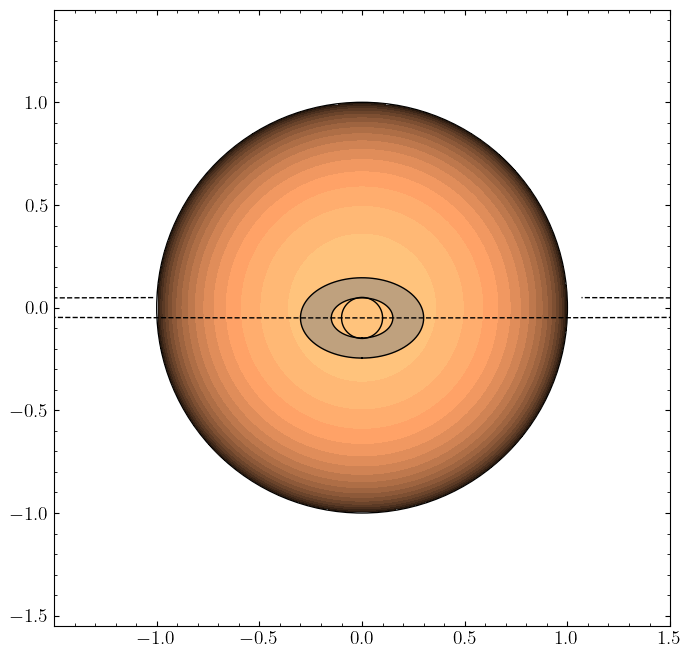
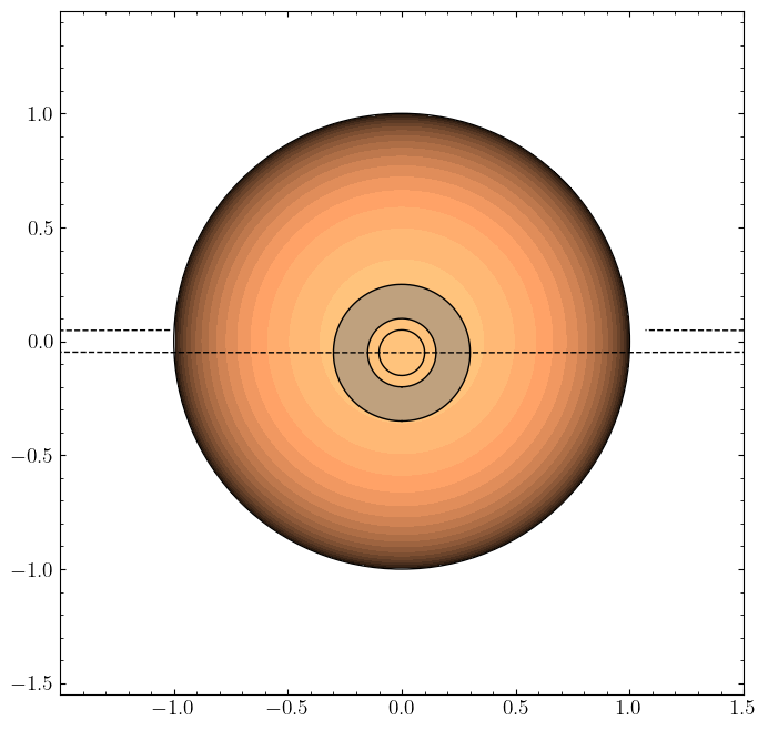
At ring_obliq = 0.05 the annulus is nearly edge-on and adds almost nothing beyond the planet’s transit; by ring_obliq \(= \pi/2\) it is face-on and blocks its full annular area.

An edge-on ring vanishes exactly

An infinitely thin ring seen perfectly edge-on projects to a line segment and blocks no flux. This limit is handled exactly (with well-defined gradients), rather than through any special-casing or clipping:

edge_on_state = dict(state)
edge_on_state["i"] = jnp.pi / 2

edge_on = RingedSystem(
    ring_inner_r=0.15,
    ring_outer_r=0.3,
    ring_obliq=0.7,
    ring_prec=0.0,
    **edge_on_state,
)
no_ring = OblateSystem(**edge_on_state)

max_diff = jnp.max(jnp.abs(edge_on.lightcurve() - no_ring.lightcurve()))
print(f"max |edge-on ringed - planet only| = {max_diff:.2e}")

max |edge-on ringed - planet only| = 2.22e-16

Gradients

RingedSystem inherits the same gradient machinery as OblateSystem: lightcurve is wrapped in a custom_vjp that computes derivatives with forward-mode differentiation under the hood (much faster than naive reverse mode for this model). Any parameter passed in the call-time dictionary can be differentiated, including all four ring parameters:

def summed_flux(params):
    return jnp.sum(decoupled.lightcurve(params))


grads = jax.grad(summed_flux)(
    {
        "ring_outer_r": jnp.array([0.3]),
        "ring_obliq": jnp.array([0.2]),
    }
)
grads

{'ring_obliq': Array([-11.88697967], dtype=float64),
 'ring_outer_r': Array([-23.11990875], dtype=float64)}

Both gradients are negative, as expected: a larger or more face-on ring blocks more light.

A note on performance

The ringed model evaluates up to five boundary-integral terms per timestep (plus the intersection tests between the planet, both ring edges, and the stellar limb), so it is substantially more expensive than the planet-only model for in-transit points – roughly an order of magnitude on a CPU. Out-of-transit points are masked and remain nearly free. See the performance notebook for measured timings of both the forward models and their gradients.